Chapter 13 Probability
You ever met anybody who was unusually certain about something? Like, even if they’re dead wrong?
I have. It was frustrating.
I spent years under the tuteledge of behaviorists. For those unfamiliar with the idea, the behaviorist philosophy of human behavior suggests every single action can be boiled down to punishments and reinforcements. Under this paradigm, you can manipulate just about any behavior just by managing the punishments and reinforcements.
Simple as that.
That brings me to my story. Her name was Jill: brown hair, blue eyes, and she seemed to float through life like Cinderella. She never stopped smiling. Or singing. Really, folks. She was ripped straight out of a fairy tale.
She really only had that one flaw: she was certain about everything, even when it could have helped her to be a bit less sure.
She was having trouble with her toddler disobeying and throwing tantrums. She was clearly venting, not asking for advice.
I usually try to shy away from offering advice when it’s not solicited. But, at that time, I was working with an autistic kid who used to disobey and throw tantrums. But, not anymore.
Why?
Because I had managed his punishments and reinforcements.
So, I offered my unsolicited advice. I don’t remember what I said, but I’m sure it was brilliant, cuz, well, it was me talking ;)
“Not going to work,” she said.
“Uh…what?”
“Not going to work.”
“Why?” I asked.
“Because kids don’t understand consequences. Not until they’re two.”
I raised an eyebrow. “I don’t think that’s tr–”
“Nope. It’s true. They don’t understand consequences. Not until they’re two.”
Yeah–no. With punishments and reinforcements, you can teach a dog to poop in the toilet. You can train a fish to read. You can train a freaking pigeon to navigate a freaking missile!
You can certainly train a toddler to obey.
But, she was certain. Argument over.
I’d hate to be her husband.
You see, fare student of mine, there is nothing in life that is certain. Some things are more probable than others. And for those who are not as hard-headed as Jill, we want to know about probability.
13.1 Why and when we need probability?
So far, all our research questions could be answered with just our dataset. But, if you ever want to generalize your results beyond the dataset, you need probability.
What sorts of questions might you ask?
I just swallowed a gallon of gasoline. What’s the probability I will die before I reach the hospital?
Or
I’ve always wanted to be kidnapped by aliens. If I shine a laser in Morse Code into the night sky, how likely is it my future captors will spot me?
Or
I’m thinking about investing in AOL.com. If I invest now, how much return on investment will I get in six months?
All these questions require us to tap in to the “phenomenal cosmic power” of probabilities.
Rather than asking why we need probability, we might ask when we need probability.
That’s a good question. (You’re really bright, you know that?)
We need probability any time we want to make inferences beyond our dataset. There are two situations where we might make inferences:
Hypothesis testing. In stats, people often use probability to make decisions about a hypothesis. For example, if Model A is more than 10 times more probable than Model B, I’m going to choose Model A. Or, if the probability that Model A is no different than Model B is less than 0.05, I will choose Model A.1 These are probability questions that only probability can answer.
Confidence/credible intervals. These intervals are used to represent our degree of uncertainty. We may not care about testing a hypothesis, but instead care about how precise our estimate of a mean is, for example.
By the way, everything we’ve done in this book up until now has not required any probability. We’ve looked at graphics. We’ve computed means and variances. We’ve even computed correlations and Cohen’s d’s. But we haven’t used probability.
Yes, it is possible to do statistics without probability.
But, the conclusions we’ve gleaned so far have been limited to what we find in our dataset. If we want to make any sort of inferences beyond our dataset, we need probability.
So, probability, old friend…it is time we meet again.
13.2 Finite Samples
Did you hear? There’s going to be a raffle. The prize? A date with Matthew McConaughey.
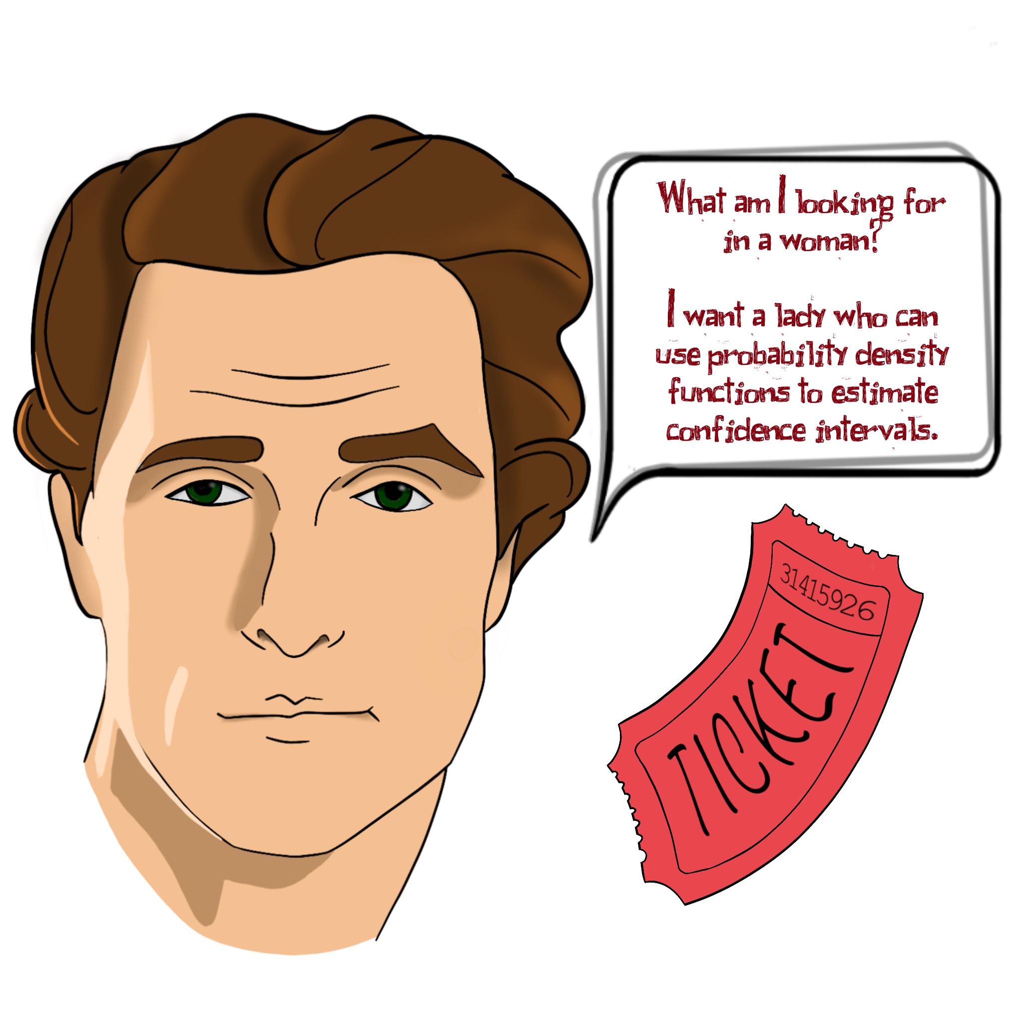
He’s so hot.
That Texas drawl…my oh my.
Where were we?
Oh yes. Raffle.
It’s a charity thing. All you have to do is pay a dollar to enter the raffle. Pay two and you get two tickets.
You know the event organizers are going to cap it at 1,000,000 tickets. Why are they capping it, you ask? Well, because it makes the sample finite, which makes my example easier. So leave me alone. (I’ll get more into finite versus infinite samples shortly).
Anyway, it’s been your dream since before you hit puberty to stare into those dreamy eyes of his. Problem is, you don’t have a whole lotta money.
So what are your chances of winning a date?
It’s simple: if you buy one ticket, it’s 1/1,000,000. Your probability is one in a million.

If you buy two, it’s 2/1,000,000
Now it’s time for a definition:
Probability: The number of cases I’m interested in divided by the total number of cases possible
Not a very tweet-worthy definition, but it’s good enough for now.
So, if you bought 10,000 tickets, you’re interested in one of those 10,000 being selected. The total number of cases includes both those you’re interested in and those you are not (which, in this case, is 1,000,000).
Probabilities range from zero to one; zero means there’s absolute certainty it did not happen. One means there’s absolute certainty is did happen. For our raffle example, a one means you bought all 1,000,000 tickets. Zero means you didn’t buy a single ticket.
Alas, this definition really only works if you can actually count the number of cases possible.
Which we can’t always do.
13.3 Infinite sets
Finite sets are countable.
Infinite sets are not.
If we do know the total number of cases, we have a finite set and we can compute a finite probability.
If we do not know the total number of cases, we have an infinite set, which is going to complicate things.
Let’s play a game. I give you a probability situation and you tell me if it contains a finite set or an infinite set.
The probability you will be selected next for a game of kickball at recess.
The probability your death will be featured on Darwin Awards
The probability you win a raffle for a free set of footie pajamas
How’d you do?
Oh yeah…I need to give you the answers.
But now I’m wasting space, so you can’t see the answers.
Alright, my editor’s yelling at me. Seems each character costs precious ink and she just docked my commission.
Wait…I wrote this book. I’ll dock your commmission!
Now, where was I?
Oh yeah.
The answers.
Don’t forget to flip the cereal box upside-down.
Question: The probability your death will be featured on Darwin Awards
The probability you win a raffle for a free set of footie pajamas
Answer: This is clearly a finite set. The total number of tickets is countable.
Now stop standing on your head. You’ll get dizzy.Like I said, you can’t always count the number of possible cases. Why?
There’s two reasons a probability question might be infinite:
The probability asks something about the future. Some questions are inherently asking about something that hasn’t yet happened. “What’s the probability Justin Beiber will win the next presidential election?” “What’s the probability I’ll catch measles tomorrow?” “What’s the probability nobody will buy my silly stats book?” To compute these sorts of probabilities requires you to project into the future, a future that cannot be counted now.
The probability asks something about a very large number of cases. Sometimes it’s either impossible or really difficult to count the number of possibilities because it’s so massive. For example, say you work at a call center. You chose this job because you thought it would be a nice way to meet guys…on the phone. You talk to a customer who has a sexy voice and you consider asking him out. What is the probability he’s a 8 or above on the CHI (Customer Hotness index, or, for the more crass, the CFI…Customer…oh, nevermind)? Well, that’s tough. We’d have to know the number of customers with CHI’s over 8, as well as the total number of customers (or at least male customers). We could collect these data, but it would be really difficult to do.
So what do we do? Are we forever doomed to leave the cosmic powers of probability untapped?
No.
When the set is infinite, we sample.
13.4 Infinite Sets and Sampling
I hate definitions, by the way.
Okay, mini rant.
I think definitions are lame because I don’t think an arbitrary name from an arbitrary person really matters. I say tow-may-toe. You say tow-mah-tow. But we could just as well call it red-round-cucumber. Or flumpbat.
But, definitions sometimes help us communicate a concept. So, please, don’t memorize the words I’m about to say, but memorize the concept.
Now, what is a population?
Population: The whole crap-ton of possible outcomes that could occur.
How’s that for precision?
(I do think that one’s tweet-worthy. Go ahead…I’ll wait).
So, if you’re wanting to know the probability this customer has a CHI of 8 or higher, your population is all the possible CHI ratings you might get.
If you’re wanting to know the probability your death will be featured on Darwin Awards, your population might be all possible ways your death might be reported.
If you’re wanting to know the probability of Beiber for President, your population could be all Americans eligible for running for President.
Alas, it’s really hard to sample the entire population. If we could, it would be a finite set and we’d be done with it. But we don’t.
So what do we do?
We sample.
Let’s define that, shall we?
Sample: A small, manageable subset of the population that we can actually access.
The basic idea is this: we collect a sample and compute our statistics. We then use the statistics from the sample to make guesses about what the population looks like.
For example, say our population is all male customers, regardless of CHI. It would be unfeasible to gather pictures from all customers, so maybe you peruse the customer database, gather a couple hundred names, look up their pictures on Facebook, then assign a CHI for each customer. You can then pretend the set is finite and compute the proportion of your sample that has a >8 CHI.
(Although, now that I think of it, you could probably just Facebook stalk the customer with the sexy voice. But that would ruin my example.)
If our sample is representative of the population, the information gleaned from the sample will probably be similar to the information from the population.
Aaaaand, time for another definition:
Representative sample: A sample that looks a whole crap-ton like the population.
Care for an example?
Say the actual customer database has an average CHI of 6.1, and 20% of the population has a CHI >8. But maybe when you sampled from the database, the database was sorted by how long they’d been a customer. So you accidentally sampled those who had been customers for a long time. And maybe all those customers were really old and lost the beauty of youth. So your sample had an average CHI of 2.2, and only 6% of the population had a CHI >8. This would be an unrepresentative sample.
It turns out, making statistical inferences only works if our sample is representative. If not, we’re kinda screwed.
That’s a pretty important point, so I’m going to fake-tweet that:
Statistical inferences to the population only work if our sample is representative of the population.
Let’s think of another example. As of the time of this writing, Donald Trump is president. Also as of this writing, Fox News viewers love Trump. Say you want to know the probability Trump will win the next election. What is your population? All eligible American voters that plan on voting. You could gather a sample by posting a poll on Fox News’ website. Now suppose you got a massive sample (maybe 1 million responses).
Would that sample be representative?
Likely not.
Why? Because those who read Fox News tend to like Trump more than the average American. You end up oversampling Trump supporters and undersampling Bieber supporters. Er…I mean, Biden supporters.
13.5 How to ensure a representative sample
Let me tell you how not to obtain a representative sample.
We can use convenience sampling.
Well, darn. Definition time again.
Convenience sample: A sample that is selected because it is easy to collect.
Let’s consider some examples:
A sample of undergraduate psychology students
A sample of those who enter a particular clinic to get treatment
A sample of your twitter followers
Depending on your population, there’s little reason to suspect convenience samples are representative samples; very seldom are convenience samples representative samples.
Unfortunately, most of psychological research is performed on convenience samples.
That’s depressing.
So if convenience samples are so rarely representative, whatever shall we do?
I’m actually not going to go into detail here, because I’m lazy. But, in summary, the best you can do is random sampling. Random sampling means that every person in the population has an equal probability of being selected.
It turns out, random sampling is really hard to do. So there are some shortcuts, including:
- Stratified random sampling
- Cluster sampling
- Purposive sampling.
If you want to know more, see my YouTube video on sampling. Go ahead. It’ll be good for you.
But let me say one more thing: sometimes it may not matter whether our sample is entirely representative.
How do you know if it matters?
Uh oh…I feel a fake-tweet coming on:
If the quirky characteristics of your sample are uncorrelated with the variables you’re studying, a representative sample doesn’t matter.
What does that mean? If your sample is unrepresentative, that means they have “quirks” that make them different from the population. If these quirks are uncorrelated with the variables your studying, your sample’s as good as representative of the population.
Remember our previous example where you inadvertently sampled a bunch of old men and measured their CHI? In this case, the quirks of your sample (old men) was correlated with the variable you wanted to study (CHI).
On the other hand, if you sorted the database by zip code, your sample would still be quirky! You’d get a whole lot of people from the east coast. But there’s no reason to suspect that those living on the east are more or less attractive than those living anywhere else. (I’ve lived on both coasts, so I should know. And I’m an excellent judge of hotness).
Anyway, enough of that sampling business. Let’s just pretend that, at this point, your sample is representative of the population, at least in all the ways that are important. If our sample looks like the population, we can make inferences from our sample to the population.
How?
Using probability density functions.
13.6 Probability Density Functions
Man, this is a lot of information. Should we take a break for a joke?
Joke time:
Why did the stoplight turn red?
Wouldn’t you turn red if you were caught changing in the middle of an intersection?!
Ah. I hope you had a good laugh. Don’t spill your laughing tears on your text. The editor went with cheap ink that’s likely to bleed.
Anyway. Where were we?
Oh yes. Matthew McConaughey. Hotness Ratings. Probability Density Functions.
Let’s say you’re trying to save your money to purchase a limited edition Beanie Baby unicorn. Let’s say you make $1,000 a day and the baby costs $25,000. How long before you can snuggle with your unicorn?
There’s two ways to calculate it.
Method 1: You can, at the end of every day, count the amount of money you have. Every day after work, you’d ask yourself,
“Is today the day? No. :(”.
“Is today the day? No. :(”.
“Is today the day? No. :(”.
“Is today the day? No. When is it going to happen?!?!?!?”
Then, on day 25, you’d say,
“Is today the day? Oh my dear goodness! It is! I never thought it’d be today! Wow! I’m so haaaaapppppppyyyyyyyyyy!”
That would be ridiculous.
You don’t need to ask yourself everyday if today is the day. You could know before you even work a single day.
All it takes is a little math:
See all the trouble you saved yourself? Rather than counting your money on 25 different occasions, you can use a mathematical equation.
Probability Density Functions (or PDFs, if you’re in the ‘in’ crowd of statisticians) are like that simple formula. They too are mathematical equations that condense a whole freak-ton of information into a simple formula. These equations can tell us the probability of every single score (though, see the note below).
Density versus probability
Probability density functions actually don’t tell you the probability of certain scores. Technically, probability isn’t defined for numeric distributions (because there are an infinite number of values for numeric variables, which means that the probability of observing any one value is technically zero). Instead, PDFs tell us about the density of a particular score. Density is basically the height of the histogram at that particular X score. However, you can use PDFs to tell you the probability of a range of scores (e.g., the probability that a score is higher than 10).
For example, here’s the probability density function for a normal distribution:
I know, it’s scary. Take a break if you need to. But really, it won’t hurt you. Actually, here’s a cute picture of kittens. Maybe that’ll help you feel better.

Back?
Good.
Now, you do not have to memorize this formula. I don’t have it memorized. I’ve got too many other things to memorize, like the BTU’s in various species of eastern US hardwoods, and the names of my children.
But notice that the formula has a couple wonky symbols:
\(\sigma\) is the standard deviation
\(\mu\) is the mean
\(x\) is the score
\(\pi\) and \(e\) are just numbers masquerading as letters
That tells us that, in order to compute the probability of every possible score we could ever obtain (i.e., \(x\)), all we need to know is the mean and standard deviation.
That’s some powerful sh$t. Srsly.
Now, back to sampling. Let’s say we have a representative sample. If so, the mean from our sample should be pretty dern close to the population mean. Also, our sample’s standard deviation should be pretty close to the population standard deviation. If that’s the case, then….
You see it, don’t you…
With only the mean and standard deviation, we can compute the probability of any freaking score we could possibly imagine. Or, we could use finite probability calculations for infinite probabilities.
That there is powerful stuff.
Right probability genie?

13.6.1 Computing Probabilities From PDFs
Let’s go ahead and compute some probabilities from a PDF. You know, just for fun. Well, I guess it’s more than just for fun. It’s also to give you some intuition about the relationship between means/standard deviations and probabilities.
So, let me forewarn you: this section is a little more technical and laden with minutia. You will never actually have to do this! R (or JASP) will do all this for you in the background. I’m just showing you for fun. Please don’t lose focus on the big picture here: the point of this section is to (a) demonstrate that you can use PDFs to compute probabilities, and (b) give you some sense of the relationship between standard deviations/probabilities.
Let’s say a local comic book store has a sample of 10,000 comic books. Also, you know that the value of these comic books is normally distributed. The owner of the comic book store says one day that he is giving these away for free, as a promotion and whatnot. Also, the owner knows the average value of each book is $25 and the standard deviation is $8. Why does he know that? I don’t know. But it makes my example easier.
Anyway, it will take about $10 of gas just to get to the comic book store. Is it worth it? Or, in other words, what is the probability you will acquire a comic book of at least a $10 value?
That’s easy to compute in R:
mean = 25
sd = 8
p.of.not.being.worth.it = pnorm(10, mean, sd)
p.of.worth.it = 1 - p.of.not.being.worth.it
p.of.worth.it
#> [1] 0.9696036So, lemme esplain. The pnorm function asks R to compute the probability of obtaining a score less than or equal to a particular value (10 in the example), under a given mean (15) and standard deviation (8). In this case, it tells us the probability of getting a comic book of $10 or less. We actually want to know the opposite of that (probability of getting a value of $10 or more). That’s why we subtract the value of p.of.not.being.worth.it from one.
Now, what’s the probability of getting a comic worth over $100? Instead of pluggin in 10, let’s plug in 100:
mean = 25
sd = 8
p.of.less.than.lots = pnorm(100, mean, sd)
p.of.mucho.mula = 1 - p.of.less.than.lots
p.of.mucho.mula
#> [1] 0With rounding error, that probability is zero. Why? Because 100 is ridiculously far from the mean!
Let’s go ahead and look at a graphic to see that:
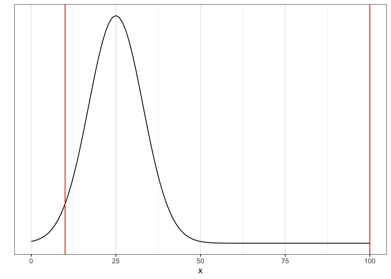
Getting a comic worth $100 or more (right red line) would be extremely rare (so much so, that the probability is very close to zero). But getting a comic worth more than $10 is much more likely.
This example assumes a mean of 25 and a standard deviation of 8, but we could use the pnorm function for any normal distribution. In fact, sometimes it’s helpful to completely disregard the mean and standard deviation. To do so, we can compute what we call a z score:
\[z = \frac{\text{score} - \text{mean}}{\text{standard deviation}}\]
A z score is able to put every single possible score (from dollars in comic books, to height, to weight, to nerdiness score) into a common scale. That scale means how many standard deviations different a particular score is from the mean. For the $10 comic book case, that would be
\(z = \frac{10 - 25}{8} = -1.875\)
This score (-1.875) says that a score of $10 is 1.875 standard deviations below the mean. Likewise, a score of 100 is 9.375 standard deviations above the mean. Also, a z-score of height of -1.875 means that one is 1.875 standard deviations below the mean of height; a z-score nerdiness score of 9.375 is 9.375 standard deviations above the mean of nerdiness.
Also, having a z-score above 1.5 on the nerdiness scale has the same probabilities as a score above 1.5 of a height scale or a 1.5 of an income scale. (As long as they’re all normally distributed).
To better give you an intuition for how z-scores map into probabilities, see the table below. Notice how a whopping 68% of scores are within 1 standard deviation of the mean! So, if your score on your next exam is 1 standard deviation above the mean, you really rocked it! Only 16% of people beat you!
| Z Scores | Probability |
|---|---|
| Between -1 and +1 | 68% |
| Between -1 and 0 | 34% |
| Above +1 | 16% |
| Between -2 and +2 | 95% |
| Above 2 | 2% |
Once again, let me emphasize the point of this section: I want to demonstrate that you can use PDFs to compute probabilities. That’s all. You’ll probably never in your life use the pnorm function in R because most statistics packages will compute these for you as part of the modeling process (without pnorm). Also, a second point of this exercise is to give you some intuition of how probabilities map into standard deviations.
So, if you’ve got that, you’re good to go. Otherwise…umm…read it again? Then send me hate mail about how dreadful that section was.
13.7 Chapter Summary
Often the research questions we might want to ask require us to reach beyond our samples. More specifically, if we want to use hypothesis testing or create confidence intervals, we need probability.
Computing probability from finite sets is easy: it is the number of instances you are interested in divided by the number of possibilities. However, most samples are infinite. Two situations that require infinite samples are when you are going to try to predict the future, or when it is too cumbersome or impossible to gather the population.
To move beyond our dataset, we sample from the population, then use probability density functions (PDFs) to make inferences. PDFs are just confusing mathematical formulas that tells us everything we could possibly want to know about the population from just the mean and standard deviation.
We also learned that we can convert scores (e.g., value of a comic book in dollars) into a common scale called a z-score. All z scores have the same probabilities, and a whopping 68% of scores fall within one standard deviation of the mean (for normal distributions).
Wicked cool.
Ready for the next chapter?
Your excitement is audible to me, even now in the distant past. So let’s get to it.
For the pedantic, yes, I know this statement is an inaccurate representation of Null Hypothesis Significance Testing. It should be, “if the probability that Model A is no different than Model B under the null hypothesis is less than 0.05, …” But, come on, I’m trying not to complicate things…yet.↩︎