Yes, simple slopes….

So….apparently this is a thing.

But I’d never heard of it until a year ago. And I didn’t understand it until last week.

“Aren’t you a quantitative psychologist?” you say…

Why yes, yes I am.

“Isn’t that basic knowledge?”

Maybe. Maybe not. I suspect my unfamiliarity with simple slopes has little to do with my prowess at maintaining a pulse on quantpsych. Rather, people like to call different things by different names.

(Don’t get me started on SPSS’s “hierarchical regression models.”)

When do you use simple slopes?

Good question!

You (typically) do a simple slopes analysis after you’ve detected a statistically significant interaction. (I almost vomited writing the words ‘statistically significant’). In other words, interactions are an afterthought, at best.

(Maybe I’ve never heard of simple slopes because, to me, interactions are never an afterthought).

Let’s look at an example, shall we? Below, is an anova summary table of the avengers dataset:

	Df	Sum Sq	Mean Sq	F value	Pr(>F)
speed	1	228840.41	228840.41	624.0194	0
superpower	1	121771.09	121771.09	332.0546	0
speed:superpower	1	83506.39	83506.39	227.7116	0
Residuals	808	296309.80	366.72	NA	NA

My oh my, how significant that interaction is.

Once our results tell us something we should have predicted in advance (i.e., an interaction is present), we now want to know the nature of the interaction. What does it look like?

That’s where simple slopes comes in.

A simple slopes analysis simply computes predictions for various levels of the data. So, we might try to see how our model predicts shots.taken (our outcome variable) for a few different values of speed and for each level of superpower (yes versus no). That might look like this (btw, this is a bad way of doing this, so don’t….):

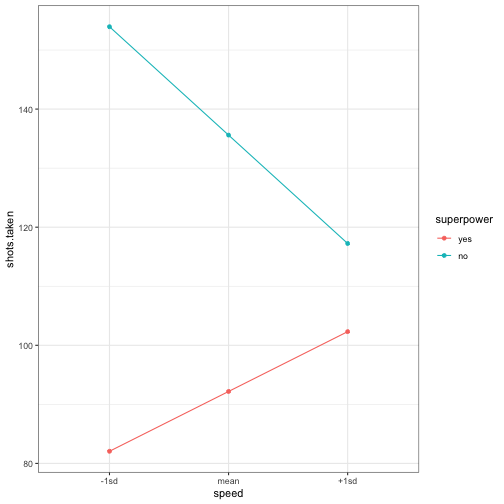
So, apparently, speed means more shots taken for non-superheroes and less shots taken for superheroes.

But, this is problematic.

Why?

Why Simple Slopes Models are Problematic

Well, there’s worse things one could do. But, this model takes a continuous variable (speed) and condenses all that rich information into just three values (-1sd, mean, +1sd). It’s not necessary. Instead, why not just plot a regular-old scatterplot (and maybe have different panels for superheroes and non-superheroes)?

By the way, this is exactly what flexplot does: where possible, it maintains the continuous nature of the data. There’s no funky coding we have to do. We don’t have to save predictions to excel then export them to another program. It just does this naturally.

Let’s go ahead and look at how to do it in JASP first, then I’ll show you how to do it in R.

Computing simple slopes with JASP’s Visual Modeling Module

It’s really so easy to do this, it shouldn’t require a tutorial. But, I’ll ablige 🙂

If you haven’t added the Visual Modeling module yet, do so by pressing the + button at the top right:

then checking the Visual Modeling Module:

(sorry….my version is in dutch for some reason…don’t ask :))

Now, import your dataset, then click on Visual Modeling at the top, and select “linear modeling” (second option)

 

Now select your predictors and your outcome:

Then you’ll have to add your interaction term under the “Model Terms” menu (or Modeltermen if you’re dutch :)). To do so, select both predictor variables, then click the right arrow:

Then look to the right.

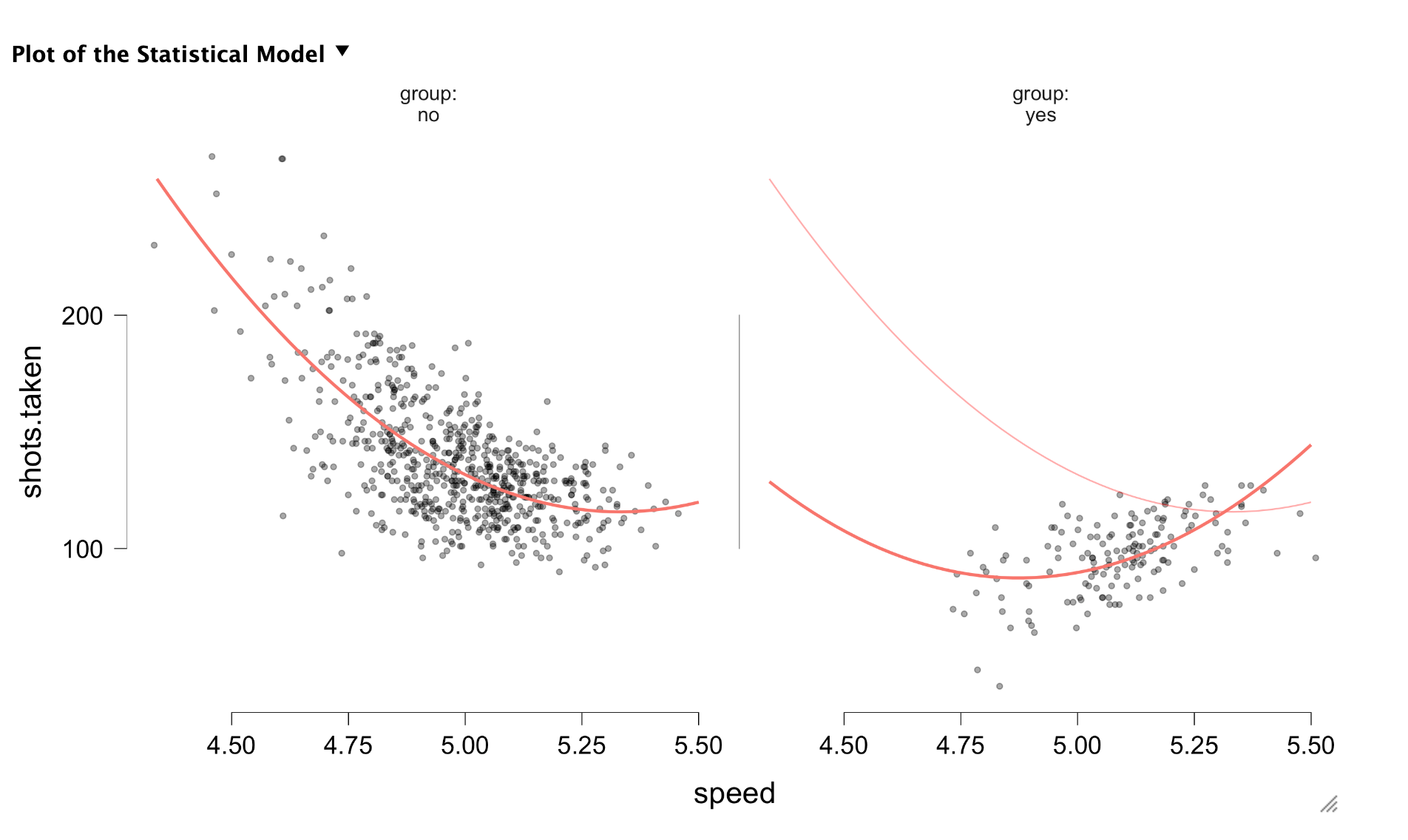
There’s your simple slopes graphic, except it doesn’t compress the data like the first figure did. And, it includes raw data so you can know if your model actually fits.

Which it doesn’t.

Let’s go ahead and add a polynomial term by first clicking “Add as a polynomial” on the speed variable:

Then click on the “Visual fitting” pane and select “Quadratic” from the menu:

And now our model has a polynomial term:

For more information on visualizing in JASP, see my article on JASP’s website or my YouTube playlist

Computing simple slopes in R with Flexplot

This is all quite easy in R, if you’re familiar with it:

require(flexplot)
data(avengers)
model = lm(shots.taken~speed+superpower + I(speed^2) + speed:superpower, data=avengers)
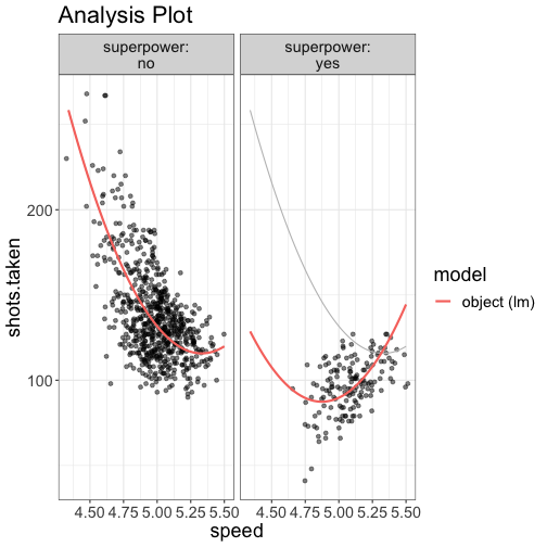
visualize(model, plot="model", ghost.line="gray")

For more information on doing this in R, see my Flexplot manual.