Well, I learned something today.
I received an email Before I share that, let me give a little background. This individual is trying to perform logistic regression using the following model:

Or, in R code:
model = glm(y~x*z, data=d, family=binomial)
Now, let’s see what this individual says:
We’ve got a significant interaction effect in our logistic regression. Now we want to break it down and interpret it using simple effects. In the attached handout on page 2, paragraph 2, (paragraph beginning “Simple slopes can be..”) the method describes testing the model 3 times with different scalings of the Z variable. One test should be with the Z variable scaled so that the mean is 0. The second test should be with the Z variable scaled at one SD above the mean. The third test is with the Z variable scales at one SD below the mean. So the interaction effect is run 3 times. The subsequent pages show examples of this process.
The problem I’ve encountered is that when I do that, the Betas, Wald, Odds ratios etc are the same for all 3 of these tests for the interaction effect. I’ve missed something. Help is needed!
(First suggestion: avoid passive voice :))
And, here is what the mentioned handout says,
Simple slopes can be tested using a macro (e.g., Andrew Hayes’ macros for SPSS and SAS (http://afhayes.com/spss-sas-and-mplus-macros-and-code.html and http://processmacro.org/index.html) or a computer method. In the computer method, the logistic model with the interaction is tested multiple times using different scalings for the Z variable. This method capitalizes on the fact that when Z is centered, the main effect for the X variable, β1, from the interaction model is a simple effect coefficient. It represents the effect of X when Z is equal to its mean, because the rescaled value z has a value of 0 when Z is equal to its mean. Rescaling Z again, where the standard deviation (sz) is subtracted, zhigh = z – sz, gives the simple effect coefficient and its significance test for X at one standard deviation above the mean of Z. The x variable scaling is unchanged, but the interaction must be computed anew, so that xzhigh = zhigh*x. The low-Z slope simple slope can be tested by rescaling Z again, this time adding one standard deviation from the mean of Z, where zlow = z + sz, and then recalculating the interaction term.
So, in summary, the text this individual is following suggests that he needs to transform Z three different ways:


Or, in R code:
z_centered = z - mean(z)
z_low = z_centered - sd(z)
z_high = z_centered + sd(z)
Then compute the significance of  for each of these of these models:


Or, in R:
mod_centered = glm(y~x*z_centered, data=d, family=binomial)
mod_low = glm(y~x*z_low, data=d, family=binomial)
mod_high = glm(y~x*z_high, data=d, family=binomial)
And, I should probably be honest; I thought the answer to his question was obvious.
And, I was wrong.
Here’s what I started to write:
… he should have identical results. As they say in stats, “statistical models are invariant to linear transformations.” That’s just a fancy way of saying you can analyze, say sexual aggression as is, or you can analyze sexual aggression + 1 and you’re going to get the same results (though the intercept will be different). I’m not clear on what this paper is suggesting. If I didn’t know better, I would think it’s suggesting exactly as Damon did. But again, that’s a silly thing to do. I suspect what they meant is to test the X effect for data where Z is approximately 1 standard deviation above the mean, then do the same for where Z is approximately 1 standard deviation below the mean. If so, then your dataset for the two tests (+/1 sd) will have smaller sample sizes than the full dataset.
But, I figured I would double-check and make sure I wasn’t deceiving myself. So, I simulated some data to verify what I was saying was correct. (This is for a regular regression, not logistic, but my conclusions would be the same either way):
require(tidyverse)
# simulate data
x = rnorm(100)
z = .2*x + rnorm(length(x), 0, sqrt(1-.2^2))
y = .4*x + .3*z + -.3*x*z + rnorm(length(x), 0, .75)
d = data.frame(y=y, x=x, z=z, z_low = z-sd(z), z_high = z+sd(z))
# fit the models
mod = lm(y~x*z, data=d)
mod_low = lm(y~x*z_low, data=d)
mod_high = lm(y~x*z_high, data=d)
# summarize p values in a table
p_centered = summary(mod)![coefficients[,4] %>% round(3) p_low = summary(mod_low)](https://quantpsych.net/wp-content/ql-cache/quicklatex.com-99f58eacce5f8e4a09a4dd6894f1d0e2_l3.png "Rendered by QuickLaTeX.com") coefficients[,4] %>% round(3)
p_high = summary(mod_high)
coefficients[,4] %>% round(3)
p_high = summary(mod_high)![coefficients[,4] %>% round(3) results = data.frame( p_low, p_centered,p_high) knitr::kable(results) </code></pre> <table> <thead> <tr> <th align="left"> </th> <th align="right">p_low</th> <th align="right">p_centered</th> <th align="right">p_high</th> </tr> </thead> <tbody> <tr> <td align="left">(Intercept)</td> <td align="right">0.000</td> <td align="right">0.208</td> <td align="right">0.018</td> </tr> <tr> <td align="left">x</td> <td align="right">0.503</td> <td align="right">0.000</td> <td align="right">0.000</td> </tr> <tr> <td align="left">z_low</td> <td align="right">0.000</td> <td align="right">0.000</td> <td align="right">0.000</td> </tr> <tr> <td align="left">x:z_low</td> <td align="right">0.000</td> <td align="right">0.000</td> <td align="right">0.000</td> </tr> </tbody> </table> Oh snap. Yeah, I goofed. Those p-values are indeed different. (Especially the one the paper said should be different--X) So, what was wrong with my logic? Well, it is true that the <em>entire</em> statistical model is invariant to linear transformations. For example, if we pulled out the R squared/F-Statistic for the whole model, we'd get: <pre><code class="r">whole_model = list(summary(mod), summary(mod_low), summary(mod_high)) %>% # string together the models map_dfr(function(x) c(x](https://quantpsych.net/wp-content/ql-cache/quicklatex.com-d600c107579e4679616fe439b3369ac5_l3.png "Rendered by QuickLaTeX.com") r.squared, x
r.squared, x![fstatistic[1])) # pull out r squared and f statistic names(whole_model) = c("R Squared", "F Statistic") knitr::kable(whole_model, digits=2) </code></pre> <table> <thead> <tr> <th align="right">R Squared</th> <th align="right">F Statistic</th> </tr> </thead> <tbody> <tr> <td align="right">0.49</td> <td align="right">30.55</td> </tr> <tr> <td align="right">0.49</td> <td align="right">30.55</td> </tr> <tr> <td align="right">0.49</td> <td align="right">30.55</td> </tr> </tbody> </table> When you toy with centering, you're not actually changing the total](https://quantpsych.net/wp-content/ql-cache/quicklatex.com-227a34115ac1ab0dffd2ec7fd1c11642_l3.png "Rendered by QuickLaTeX.com") R^2$ (or even the semi-partials), you're just adjusting the values of the slopes/intercept. Since slopes/intercepts are inextricably tied to the actual values of the variables, changing the values of the variables will modify the slopes/intercepts. Since p-values test the deviation of each slope from zero, you will see different p-values for the slopes/intercept.
I find this approach very confusing, btw.
What do I suggest instead?
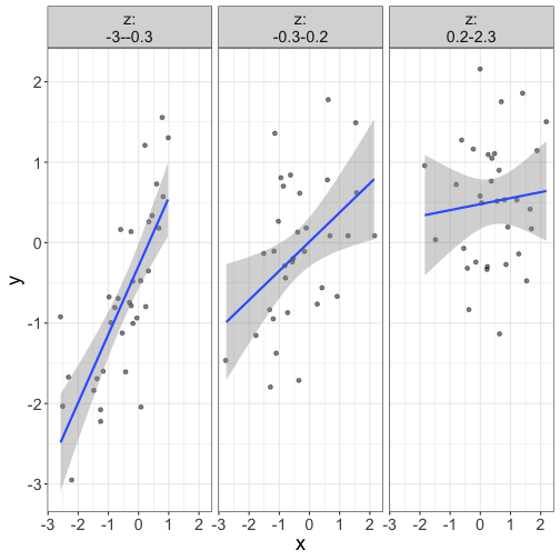
Just plot the thing. Who cares about significance?
R^2$ (or even the semi-partials), you're just adjusting the values of the slopes/intercept. Since slopes/intercepts are inextricably tied to the actual values of the variables, changing the values of the variables will modify the slopes/intercepts. Since p-values test the deviation of each slope from zero, you will see different p-values for the slopes/intercept.
I find this approach very confusing, btw.
What do I suggest instead?
Just plot the thing. Who cares about significance?
require(flexplot)
flexplot(y~x | z, data=d, method="lm")